Case study 2
Summary
The clinical trial example used in this case study is based on a Phase III trial that was conducted to evaluate the efficacy and safety of brexpiprazole, a novel treatment for schizophrenia (Correll et al., 2015). The patient population in the case study will include patients with schizophrenia who experience an acute exacerbation. The patients will be treated for 6 weeks and will be randomly assigned to a low dose of the experimental treatment (Dose L), high dose of the experimental treatment (Dose H) or placebo. An unbalanced design with a 1:2:2 randomization scheme will be employed in the trial. The use of unequal randomization helps provide more information on the treatment’s safety profile and facilitates patient enrollment since patients are more likely to be allocated to an active treatment.
The case study presents a multiplicity problem with two sources of multiplicity. The two dose-placebo comparisons (Dose L versus placebo and Dose H versus placebo) will serve as the first source of multiplicity. In addition to that, the efficacy of the experimental treatment will be evaluated using two ordered clinical endpoints:
-
Primary endpoint: Change from baseline in the Positive and Negative Syndrome Scale (PANSS) total score.
-
Key secondary endpoint: Change from baseline in the Clinical Global Impressions Severity Scale (CGI-S) score.
Note that lower values of the PANSS total score and CGI-S score are associated with improvement and thus negative changes indicate a beneficial treatment effect. The key secondary endpoint provides supportive evidence of treatment efficacy and significant findings based on both endpoints can be presented in the product label. The analysis of the primary and secondary endpoints defines the second source of multiplicity in this trial.
Define a Data Model
In this case study, two clinical endpoints are evaluated for each patient (change from baseline in the PANSS total score and change from baseline on the CGI-S score) and thus a bivariate distribution needs to be specified for each patient’s outcome in the data model. A bivariate normal distribution is defined using the MVNormalDist method in the OutcomeDist object. For each sample and each treatment effect scenario, the parameters of this bivariate distribution as well as the correlation matrix need to be defined. Parameters of the bivariate normal distribution for each expected scenarios are provided in the following table. Finally, the correlation between the two endpoints is set to 0.5.
| Endpoint | Outcome parameter set | Placebo | Dose L | Dose H |
|---|---|---|---|---|
| PANSS total score (mean (SD)) | ||||
| Scenario 1 | -12 (20) | -18 (20) | -20 (20) | |
| Scenario 2 | -12 (20) | -18 (20) | -18 (20) | |
| Scenario 3 | -12 (20) | -18 (20) | -20 (20) | |
| Scenario 4 | -12 (20) | -18 (20) | -18 (20) | |
| CGI-S score (mean (SD)) | ||||
| Scenario 1 | -0.8 (1) | -1.1 (1) | -1.1 (1) | |
| Scenario 2 | -0.8 (1) | -1.1 (1) | -1.1 (1) | |
| Scenario 3 | -0.8 (1) | -1.2 (1) | -1.2 (1) | |
| Scenario 4 | -0.8 (1) | -1.2 (1) | -1.2 (1) |
The outcome parameters are specified using the following R code.
# Correlation between two endpoints
corr.matrix = matrix(c(1.0, 0.5,
                       0.5, 1.0), 2, 2)

# Outcome parameters - Scenario 1
outcome.placebo.sc1 = parameters(par = parameters(parameters(mean = -12, sd = 20),
                                                  parameters(mean = -0.8, sd = 1)),
                                 corr = corr.matrix)

outcome.dosel.sc1 = parameters(par = parameters(parameters(mean = -18, sd = 20),
                                                parameters(mean = -1.1, sd = 1)),
                               corr = corr.matrix)

outcome.doseh.sc1 = parameters(par = parameters(parameters(mean = -20, sd = 20),
                                                parameters(mean = -1.1, sd = 1)),
                               corr = corr.matrix)

# Outcome parameters - Scenario 2
outcome.placebo.sc2 = parameters(par = parameters(parameters(mean = -12, sd = 20),
                                                  parameters(mean = -0.8, sd = 1)),
                                 corr = corr.matrix)

outcome.dosel.sc2 = parameters(par = parameters(parameters(mean = -18, sd = 20),
                                                parameters(mean = -1.1, sd = 1)),
                               corr = corr.matrix)

outcome.doseh.sc2 = parameters(par = parameters(parameters(mean = -18, sd = 20),
                                                parameters(mean = -1.1, sd = 1)),
                               corr = corr.matrix)

# Outcome parameters - Scenario 3
outcome.placebo.sc3 = parameters(par = parameters(parameters(mean = -12, sd = 20),
                                                  parameters(mean = -0.8, sd = 1)),
                                 corr = corr.matrix)

outcome.dosel.sc3 = parameters(par = parameters(parameters(mean = -18, sd = 20),
                                                parameters(mean = -1.2, sd = 1)),
                               corr = corr.matrix)

outcome.doseh.sc3 = parameters(par = parameters(parameters(mean = -20, sd = 20),
                                                parameters(mean = -1.2, sd = 1)),
                               corr = corr.matrix)

# Outcome parameters - Scenario 4
outcome.placebo.sc4 = parameters(par = parameters(parameters(mean = -12, sd = 20),
                                                  parameters(mean = -1.2, sd = 1)),
                                 corr = corr.matrix)

outcome.dosel.sc4 = parameters(par = parameters(parameters(mean = -18, sd = 20),
                                                parameters(mean = -1.2, sd = 1)),
                               corr = corr.matrix)

outcome.doseh.sc4 = parameters(par = parameters(parameters(mean = -18, sd = 20),
                                                parameters(mean = -1.2, sd = 1)),
                               corr = corr.matrix)
Also, unlike Case study 1, this case
study utilized an unbalanced design with a 1:2:2 randomization scheme. The
number of patients in each trial arm, i.e., in each sample, is specified within
each Sample object.
# Data model
mult.cs2.data.model = DataModel() +
  OutcomeDist(outcome.dist = "MVNormalDist") +
  Sample(id = c("Placebo - E1", "Placebo - E2"),
         outcome.par = parameters(outcome.placebo.sc1,
                                  outcome.placebo.sc2,
                                  outcome.placebo.sc3,
                                  outcome.placebo.sc4),
         sample.size = 100) +
  Sample(id = c("Dose L - E1", "Dose L - E2"),
         outcome.par = parameters(outcome.dosel.sc1,
                                  outcome.dosel.sc2,
                                  outcome.dosel.sc3,
                                  outcome.dosel.sc4),
         sample.size = 200) +
  Sample(id = c("Dose H - E1", "Dose H - E2"),
         outcome.par = parameters(outcome.doseh.sc1,
                                  outcome.doseh.sc2,
                                  outcome.doseh.sc3,
                                  outcome.doseh.sc4),
         sample.size = 200)
Define an Analysis Model
The statistical tests carried out in the trial as well as the candidate multiplicity adjustments are specified in the analysis model.
As both endpoints follow a normal distribution, the two treatment comparisons for each endpoint will be
carried out based on a two-sample t-test. This means that four Test objects
need to be defined in the AnalysisModel object. It is worth to be noted that as lower values for each endpoint represents an improvement, the active dose must be placed in the first position of the samples argument of the Test objects.
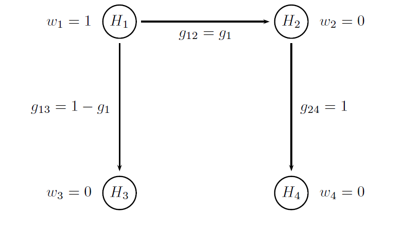
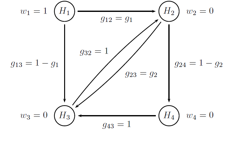
Both multiplicity adjustments are based on Bonferroni-based chain procedures, and each procedure is uniquely defined by the alpha-allocation and alpha-propagation rules. The difference between Procedure B1 and Procedure B2 lies in the specification of the alpha-propagation rule, i.e., the set of transition parameters. These procedures are represented in the following figures.
The figure below provides a visual summary of the testing strategy used in this clinical trial. The circles in this figure denote the four null hypotheses of interest:
-
H1: Null hypothesis of no difference between Dose L and placebo with respect to Endpoint 1.
-
H2: Null hypothesis of no difference between Dose H and placebo with respect to Endpoint 1.
-
H3: Null hypothesis of no difference between Dose L and placebo with respect to Endpoint 2.
-
H4: Null hypothesis of no difference between Dose H and placebo with respect to Endpoint 2.
To specify the procedure-specific alpha-propagation rules, two objects are introduced below to pass the hypothesis weights and transition parameters to the multiplicity adjustment procedures:
-
chain.weightdefines a vector of initial hypothesis weights, i.e., W1 in Procedure B1 and W2 in Procedure B2. -
chain.transitiondefines a matrix of transition parameters, i.e., T1 in Procedure B1 and T2 in Procedure B2.
Note that the transition parameters used in these procedures are computed using the optimal values of the target parameters, i.e. g1 = 0.8 in Procedure B1 and g1 = 1 and g2 = 0 in Procedure B2.
# Parameters of the Procedure B1
# Vector of hypothesis weights
chain.weight = c(1, 0, 0, 0)

# Matrix of transition parameters
chain.transition = matrix(c(0, 0.8, 0.2, 0,
                            0, 0, 0, 1,
                            0, 0, 0, 0,
                            0, 0, 0, 0), 4, 4, byrow = TRUE)

# MultAdjProc
mult.adj1 = MultAdjProc(proc = "ChainAdj",
                        par = parameters(weight = chain.weight,
                                         transition = chain.transition))


# Parameters of the Procedure B2
# Vector of hypothesis weights
chain.weight = c(1, 0, 0, 0)

# Matrix of transition parameters
chain.transition = matrix(c(0, 1, 0, 0,
                            0, 0, 0, 1 ,
                            0, 1, 0, 0,
                            0, 0, 1, 0), 4, 4, byrow = TRUE)

# MultAdjProc
mult.adj2 = MultAdjProc(proc = "ChainAdj",
                        par = parameters(weight = chain.weight,
                                         transition = chain.transition))
It is important to note that, as before, the test order in the AnalysisModel
object is important to ensure that the alpha-allocation and alpha-propagation rules
are applied correctly.
# Analysis model
mult.cs2.analysis.model =
  AnalysisModel() +
  MultAdj(mult.adj1,mult.adj2) +
  Test(id = "Placebo vs Dose H - E1",
       samples = samples("Dose H - E1", "Placebo - E1"),
       method = "TTest") +
  Test(id = "Placebo vs Dose L - E1",
       samples = samples("Dose L - E1", "Placebo - E1"),
       method = "TTest") +
  Test(id = "Placebo vs Dose H - E2",
       samples = samples("Dose H - E2", "Placebo - E2"),
       method = "TTest") +
  Test(id = "Placebo vs Dose L - E2",
       samples = samples("Dose L - E2", "Placebo - E2"),
       method = "TTest")
Define an Evaluation Model
The marginal, weighted and disjunctive power criteria utilized in this cases
study are specified in the EvaluationModel object using built-in functions.
However, two custom functions need to be developed for the subset disjunctive power criterion and partition-based weighted criterion as shown below.
# Custom evaluation criterion: Subset disjunctive power
mult.cs2.SubsetDisjunctivePower = function(test.result, statistic.result, parameter) {

  alpha = parameter$alpha

  # Outcome: Reject (H1 or H2) and (H3 or H4)
  power = mean(((test.result[,1] <= alpha) | (test.result[,2] <= alpha)) &
                 ((test.result[,3] <= alpha) | (test.result[,4] <= alpha)))

  return(power)
}

# Custom evaluation criterion: Partition-based weighted power
mult.cs2.PartitionBasedWeightedPower = function(test.result, statistic.result, parameter) {

  # Parameters
  alpha = parameter$alpha
  weight = parameter$weight

  # Outcomes
  # Outcome1: reject exactly one hypothesis in the primary family
  outcome1 = ((test.result[,1] <= alpha) + (test.result[,2] <= alpha)) == 1
  # Outcome2: reject both hypotheses in the primary family and less than two in the secondary family
  outcome2 = (((test.result[,1] <= alpha) + (test.result[,2] <= alpha)) == 2) &
    (((test.result[,3] <= alpha) + (test.result[,4] <= alpha)) <= 1)
  # Outcome3: reject both hypotheses in the primary and secondary families
  outcome3 = ((test.result[,1] <= alpha) & (test.result[,2] <= alpha) & (test.result[,3] <= alpha) & (test.result[,4] <= alpha))

  # Weighted power
  power = mean(outcome1) * weight[1] + mean(outcome2) * weight[2] + mean(outcome3) * weight[3]

  return(power)
}
Finally, the built-in and custom criterion functions are incorporated into
the EvaluationModel object.
# Evaluation model
mult.cs2.evaluation.model = EvaluationModel() +
  Criterion(id = "Marginal power",
            method = "MarginalPower",
            tests = tests("Placebo vs Dose H - E1",
                          "Placebo vs Dose L - E1",
                          "Placebo vs Dose H - E2",
                          "Placebo vs Dose L - E2"),
            labels = c("Placebo vs Dose H - E1",
                       "Placebo vs Dose L - E1",
                       "Placebo vs Dose H - E2",
                       "Placebo vs Dose L - E2"),
            par = parameters(alpha = 0.025)) +
  Criterion(id = "Disjunctive power",
            method = "DisjunctivePower",
            tests = tests("Placebo vs Dose H - E1",
                          "Placebo vs Dose L - E1",
                          "Placebo vs Dose H - E2",
                          "Placebo vs Dose L - E2"),
            labels = "Disjunctive power",
            par = parameters(alpha = 0.025)) +
  Criterion(id = "Subset Disjunctive power",
            method = "mult.cs2.SubsetDisjunctivePower",
            tests = tests("Placebo vs Dose H - E1",
                          "Placebo vs Dose L - E1",
                          "Placebo vs Dose H - E2",
                          "Placebo vs Dose L - E2"),
            labels = "Subset Disjunctive power",
            par = parameters(alpha = 0.025)) +
  Criterion(id = "Weighted power",
            method = "WeightedPower",
            tests = tests("Placebo vs Dose H - E1",
                          "Placebo vs Dose L - E1",
                          "Placebo vs Dose H - E2",
                          "Placebo vs Dose L - E2"),
            labels = "Weighted power (v1 = 0.4, v2 = 0.4, v3 = 0.1, v4 = 0.1)",
            par = parameters(alpha = 0.025,
                             weight = c(0.4, 0.4, 0.1, 0.1))) +
  Criterion(id = "Partition-based weighted power",
            method = "mult.cs2.PartitionBasedWeightedPower",
            tests = tests("Placebo vs Dose H - E1",
                          "Placebo vs Dose L - E1",
                          "Placebo vs Dose H - E2",
                          "Placebo vs Dose L - E2"),
            labels = "Partition-based weighted power (v1 = 0.20, v2 = 0.35, v3 = 0.45)",
            par = parameters(alpha = 0.025,
                             weight = c(0.20, 0.35, 0.45)))
Perform Clinical Scenario Evaluation
Using the data, analysis and evaluation models, simulation-based Clinical Scenario Evaluation is performed by calling the CSE function:
# Simulation Parameters
mult.cs2.sim.parameters =  SimParameters(n.sims = 100000,
                                         proc.load = "full",
                                         seed = 42938001)

# Perform clinical scenario evaluation
mult.cs2.results = CSE(mult.cs2.data.model,
                       mult.cs2.analysis.model,
                       mult.cs2.evaluation.model,
                       mult.cs2.sim.parameters)
Download
Click on the icons below to download the R code used in this case study and report that summarizes the results of Clinical Scenario Evaluation: