Case study 3

Summary

The clinical trial example used in this case study is based on the panitumumab trial in a population of patients with metastatic colorectal cancer (Amado et al., 2008). Using the same patient population, consider a Phase III trial for a novel treatment versus control (best supportive care) that utilizes a balanced design with a 1:1 randomization scheme. The treatment is a fully human antibody against the EGFR (epidermal growth factor receptor) and is expected to benefit mostly patients in a pre-specified subset. This subset is defined based on each patient’s KRAS (Kirsten rat sarcoma viral oncogene homolog) status and includes patients with wild-type KRAS. These patients will be referred to as biomarker-positive patients and patients with a mutated KRAS status will be referred to as biomarker-negative patients. For simplicity, it will be assumed that the KRAS status can be ascertained in all patients. The treatment effect in this two-arm trial will be evaluated based on progression-free survival (PFS).

The decision-making rules will be set up using the influence and interaction conditions defined in Section 3.2.3 of the Clinical Trial Optimization Using R.

The influence condition has been defined in Case study 2. Additional restrictions based on the influence condition as well as the interaction condition are required in a more general setting with three potential efficacy claims (broad, restricted and enhanced claims) to prevent illogical conclusions.

Beginning with a basic decision rule for formulating efficacy claims based on statistical considerations, the trial’s sponsor can consider pursuing the enhanced claim of a beneficial effect in the overall population as well as the selected subpopulation (combination of the broad and restricted claims) if the two null hypotheses of interest (H0 and H+) are simultaneously rejected. It is immediately clear that this rule does not account for the influence condition and, as a consequence, may lead to erroneous conclusions discussed above. Another potential problem with this naive rule is that the enhanced claim can be recommended even if the treatment effect is homogeneous across the biomarker-positive and biomarker-negative subsets. This may happen if the biomarker that was believed to have predictive properties turned out to be non-informative.

To address the limitations of the basic decision rule, the interaction condi- tion needs to be applied in conjunction with the influence condition as shown in the Figure below:

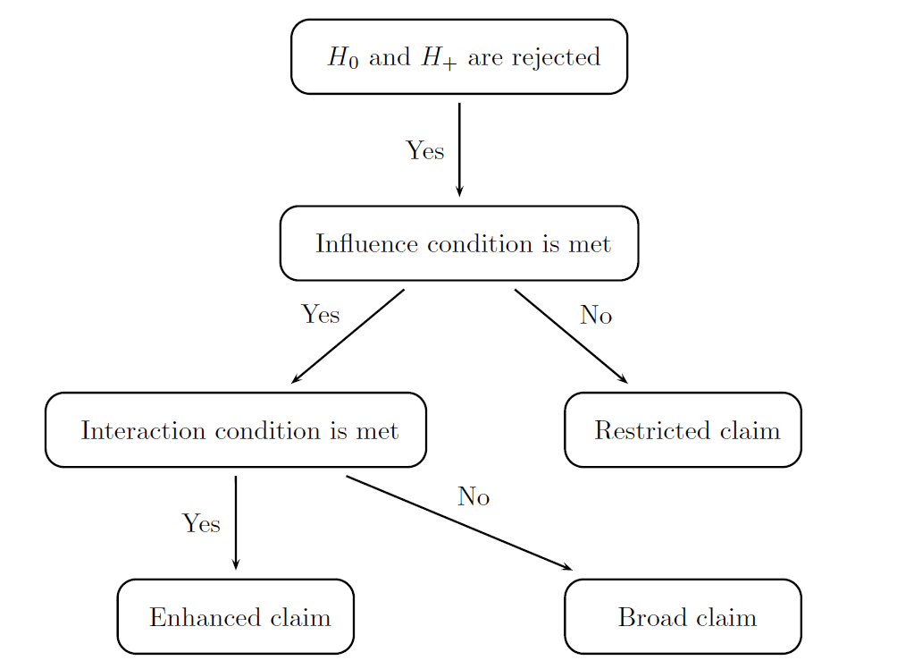
This figure defines the recommended set of decision rules for trials with three potential claims. The influence and interaction conditions are applied sequentially. The latter assesses the degree of treatment-by-biomarker interaction or strength of a differential effect in the biomarker-positive and biomarker-negative subgroups. The condition is satisfied if there is a clinically important interaction that supports the conclusion that the treatment provides a substantial additional benefit in patients with a biomarker-positive status compared to patients in the overall population. The interaction condition can be assessed using any treatment-by-biomarker interaction test. This condition can be defined using a simple test based on the ratio of the observed effect sizes in the biomarker-positive and biomarker-negative subgroups (i.e., the interaction condition is satisfied if this ratio is greater than a pre-defined threshold).

The figure shows that the enhanced claim can be made only if the interaction condition is satisfied. If no differential effect is observed and thus the interaction condition is not met, the biomarker is not useful in terms of predicting patients who experience enhanced benefit. In this case the best course of action is to focus on treatment effectiveness in the overall population of patients and pursue the broad claim.

Define a Data Model

A data model specifies a scheme for generating individual patients’ data in the set of pre-defined samples, i.e., non-overlapping homogeneous groups of patients, in a clinical trial. In this case study, the overall population of patients is naturally split into four samples that are defined as follows:

Sample 1 (Placebo Bio-Neg) includes biomarker-negative patients in the placebo arm.
Sample 2 (Placebo Bio-Pos) includes biomarker-positive patients in the placebo arm.
Sample 3 (Treatment Bio-Neg) includes biomarker-negative patients in the treatment arm.
Sample 4 (Treatment Bio-Pos) includes biomarker-positive patients in the treatment arm.

Using this definition of samples, the trial’s sponsor can model the fact that the treatment’s effect is most pronounced in patients with a biomarker-positive status.

For each sample in the data model, the parameters of the outcome distribution (i.e., hazard rate) defined in the following Table are listed in a single set of outcome parameters.

Sample	Median time (months)	Hazard rate
Placebo Bio-Neg	7.5	0.092
Placebo Bio-Pos	7.5	0.092
Treatment Bio-Neg	8.5	0.082
Treatment Bio-Pos	12.5	0.055

The outcome parameters are specified using the following R code.

# Outcome parameters
outcome.placebo.neg = parameters(rate = log(2)/7.5)
outcome.treatment.neg = parameters(rate = log(2)/8.5)
outcome.placebo.pos = parameters(rate = log(2)/7.5)
outcome.treatment.pos = parameters(rate = log(2)/12.5)

It is important to note that, if no censoring mechanism is specified in a data model with a time-to-event endpoint, all patients will reach the endpoint of interest (i.e., progression) and thus the number of patients will be equal to the number of events. Using this property, it is sufficient to define the number of patients in each sample, according to the prevalence of biomarker-negative and biomarker-positive patients. The prevalence of biomarker-positive patients in the general population (prevalence.pos) is set to 0.55.

# Sample size parameters
prevalence.pos = 0.55
sample.size.total = 270

sample.size.placebo.neg = round(((1-prevalence.pos) / 2) * sample.size.total)
sample.size.placebo.pos = round((prevalence.pos / 2 * sample.size.total))
sample.size.treatment.neg = round(((1-prevalence.pos) / 2) * sample.size.total)
sample.size.treatment.pos = round((prevalence.pos / 2 * sample.size.total))

Finally, the data model can be set up by initializing the DataModel object and adding each component to it. The outcome distribution is defined using the OutcomeDist object with the ExpoDist distribution. The data model is shown below.

# Data model
subgroup.cs3.data.model = 
  DataModel() +
  OutcomeDist(outcome.dist = "ExpoDist") +
  Sample(id = "Placebo Bio-Neg",
         sample.size = sample.size.placebo.neg,
         outcome.par = parameters(outcome.placebo.neg)) +
  Sample(id = "Placebo Bio-Pos",
         sample.size = sample.size.placebo.pos,
         outcome.par = parameters(outcome.placebo.pos)) +
  Sample(id = "Treatment Bio-Neg",
         sample.size = sample.size.treatment.neg,
         outcome.par = parameters(outcome.treatment.neg)) +
  Sample(id = "Treatment Bio-Pos",
         sample.size = sample.size.treatment.pos,
         outcome.par = parameters(outcome.treatment.pos))

By default, the outcome type is set to fixed, which means that a design with a fixed patient follow-up is assumed even though the primary endpoint in this clinical trial is a time-to-event endpoint. This is due to the fact that, as was explained earlier, no censoring is assumed in this trial and all patients are followed until the event of interest (disease progression) is observed. In the presence of censoring, the outcome type will be set to event and the design parameters, e.g., length of the enrollment and follow-up periods, will need to be specified as well.

Define an Analysis Model

The analysis model in this clinical trial is very similar to the one defined in Case study 2. The only components of the model that need to be modified are the statistical method utilized in the primary analysis (method = "LogrankTest") and method for computing the effect size in the biomarker-negative subpopulation (method = "EffectSizeEventStat"). In addition, the ratio of effect sizes between the biomarker-positive and biomarker-negative subpopulations needs to be computed. This is accomplished by specifying a Statistic object with the RatioEffectSizeEventStat method. This method computes the ratio of effect sizes for exponentially distributed endpoints.

# Analysis model
subgroup.cs3.analysis.model = 
  AnalysisModel() +
  Test(id = "OP test",
       samples = samples(c("Placebo Bio-Neg", "Placebo Bio-Pos"),
                         c("Treatment Bio-Neg", "Treatment Bio-Pos")),
       method = "LogrankTest") +
  Test(id = "Bio-Pos test",
       samples = samples("Placebo Bio-Pos", 
                         "Treatment Bio-Pos"),
       method = "LogrankTest") +
  Statistic(id = "Effect Size in Bio-Neg", 
            samples = samples("Placebo Bio-Neg", "Treatment Bio-Neg"),
            method = "EffectSizeEventStat") +
  Statistic(id = "Ratio Effect Size Bio-Pos vs Bio-Neg", 
            samples = samples("Placebo Bio-Pos", 
                              "Treatment Bio-Pos", 
                              "Placebo Bio-Neg", 
                              "Treatment Bio-Neg"),
            method = "RatioEffectSizeEventStat")   +
  MultAdjProc(proc = "HochbergAdj",
              par = parameters(weight = c(0.8, 0.2)))

Define an Evaluation Model

As in the evaluation model used in Case study 2, custom functions need to be written to support the evaluation of the probabilities of the individual claims and weighted power. Note that the definitions of broad, restricted and enhanced claims need to be updated to account for the interaction condition (see Summary). As an illustration, a custom function for computing weighted power (subgroup.cs3.WeightedPower) is defined below. The statistic.result argument in the subgroup.cs3.WeightedPower function is a matrix containing the value of the effect size in the biomarker-negative subpopulation and the ratio of effect sizes between the two subpopulations.

# Custom evaluation criterion based on weighted power
subgroup.cs3.WeightedPower = function(test.result, statistic.result, parameter)  {
  
  alpha = parameter$alpha
  v1 = parameter$v1
  v2 = parameter$v2
  v3 = parameter$v3
  influence_threshold = parameter$influence_threshold
  interaction_threshold = parameter$interaction_threshold
  
  
  # Broad claim: (1) Reject OP test but not Bio-Pos or (2) Reject OP and Bio-Pos test and influence condition is met but the interaction condition is not met
  broad.claim = ((test.result[,1] <= alpha & test.result[,2] > alpha) | 
                   (test.result[,1] <= alpha & test.result[,2] <= alpha & statistic.result[,1] >= influence_threshold & statistic.result[,2] < interaction_threshold))
  
  # Restricted claim: (1) Reject Bio-Pos test but not OP or (2) Reject Bio-Pos and OP test and influence not met
  restricted.claim = ((test.result[,1] > alpha & test.result[,2] <= alpha) | 
                        (test.result[,1] <= alpha & test.result[,2] <= alpha & statistic.result[,1] < influence_threshold))
  
  # Enhanced claim: (1) Reject Bio-Pos and OP test or reject both and influence not met
  enhanced.claim = ((test.result[,1] <= alpha & test.result[,2] <= alpha & statistic.result[,1] >= influence_threshold & statistic.result[,2] >= interaction_threshold))
  
  power = v1 * mean(broad.claim) + v2 * mean(restricted.claim) + v3 * mean(enhanced.claim)
  
  return(power)
}

A similar approach can be applied to create a custom function for computing the marginal probability of a broad, restricted and enhanced claims. These functions are defined below.

# Custom evaluation criterion based on the probability of a broad claim
subgroup.cs3.BroadClaimPower = function(test.result, statistic.result, parameter)  {
  
  alpha = parameter$alpha
  influence_threshold = parameter$influence_threshold
  interaction_threshold = parameter$interaction_threshold
  
  # Broad claim: (1) Reject OP test but not Bio-Pos or (2) Reject OP and Bio-Pos test and influence condition is met but the interaction condition is not met
  broad.claim = ((test.result[,1] <= alpha & test.result[,2] > alpha) | (test.result[,1] <= alpha & test.result[,2] <= alpha & statistic.result[,1] >= influence_threshold & statistic.result[,2] < interaction_threshold))
  
  power = mean(broad.claim)
  
  return(power)
}

# Custom evaluation criterion based on the probability of a restricted claim
subgroup.cs3.RestrictedClaimPower = function(test.result, statistic.result, parameter)  {
  
  alpha = parameter$alpha
  influence_threshold = parameter$influence_threshold
  
  # Restricted claim: (1) Reject Bio-Pos test but not OP or (2) Reject Bio-Pos and OP test and influence not met
  restricted.claim = ((test.result[,1] > alpha & test.result[,2] <= alpha) | (test.result[,1] <= alpha & test.result[,2] <= alpha & statistic.result[,1] < influence_threshold))
  
  power = mean(restricted.claim)
  
  return(power)
}

# Custom evaluation criterion based on the probability of an enhanced claim
subgroup.cs3.EnhancedClaimPower = function(test.result, statistic.result, parameter)  {
  
  alpha = parameter$alpha
  influence_threshold = parameter$influence_threshold
  interaction_threshold = parameter$interaction_threshold
  
  # Enhanced claim: (1) Reject Bio-Pos and OP test or reject both and influence not met
  enhanced.claim = ((test.result[,1] <= alpha & test.result[,2] <= alpha & statistic.result[,1] >= influence_threshold & statistic.result[,2] >= interaction_threshold))
  
  power = mean(enhanced.claim)
  
  return(power)
}

The evaluation model is presented below. The influence threshold (influence_threshold) and interaction threshold (interaction_threshold) are set to their optimal values, i.e., 0.15 and 1.5, respectively, in the computation of the probabilities of the three claims of interest and weighted power.

subgroup.cs3.evaluation.model = 
  EvaluationModel() +
  Criterion(id = "Marginal power",
            method = "MarginalPower",
            tests = tests("OP test", "Bio-Pos test"),
            labels = c("OP test","Bio-Pos test"),
            par = parameters(alpha = 0.025)) + 
  Criterion(id = "Disjunctive power",
            method = "DisjunctivePower",
            tests = tests("OP test", "Bio-Pos test"),
            labels = c("Disjunctive power"),
            par = parameters(alpha = 0.025)) +
  Criterion(id = "Weighted power",
            method = "subgroup.cs3.WeightedPower",
            tests = tests("OP test", "Bio-Pos test"),
            statistics = statistics("Effect Size in Bio-Neg",
                                    "Ratio Effect Size Bio-Pos vs Bio-Neg"),
            labels = c("Weighted power (with conditions)"),
            par = parameters(alpha = 0.025, 
                             v1 = 1 / (2 * (1 + prevalence.pos)), 
                             v2 = prevalence.pos / (2 * (1 + prevalence.pos)),
                             v3 = 1/2,
                             influence_threshold = 0.15,
                             interaction_threshold = 1.5)) + 
  Criterion(id = "Probability of a broad claim",
            method = "subgroup.cs3.BroadClaimPower",
            tests = tests("OP test", "Bio-Pos test"),
            statistics = statistics("Effect Size in Bio-Neg",
                                    "Ratio Effect Size Bio-Pos vs Bio-Neg"),
            labels = c("Probability of a broad claim"),
            par = parameters(alpha = 0.025, 
                             influence_threshold = 0.15,
                             interaction_threshold = 1.5)) + 
  Criterion(id = "Probability of a restricted claim",
            method = "subgroup.cs3.RestrictedClaimPower",
            tests = tests("OP test", "Bio-Pos test"),
            statistics = statistics("Effect Size in Bio-Neg",
                                    "Ratio Effect Size Bio-Pos vs Bio-Neg"),
            labels = c("Probability of a restricted claim"),
            par = parameters(alpha = 0.025, 
                             influence_threshold = 0.15,
                             interaction_threshold = 1.5)) + 
  Criterion(id = "Probability of an enhanced claim",
            method = "subgroup.cs3.EnhancedClaimPower",
            tests = tests("OP test", "Bio-Pos test"),
            statistics = statistics("Effect Size in Bio-Neg",
                                    "Ratio Effect Size Bio-Pos vs Bio-Neg"),
            labels = c("Probability of an enhanced claim"),
            par = parameters(alpha = 0.025, 
                             influence_threshold = 0.15,
                             interaction_threshold = 1.5))

Perform Clinical Scenario Evaluation

Using the data, analysis and evaluation models, simulation-based Clinical Scenario Evaluation is performed by calling the CSE function:

# Simulation Parameters
subgroup.cs3.sim.parameters = SimParameters(n.sims = 100000, 
                                            proc.load = "full", 
                                            seed = 42938001)

# Perform clinical scenario evaluation
subgroup.cs3.results = CSE(subgroup.cs3.data.model,
                           subgroup.cs3.analysis.model,
                           subgroup.cs3.evaluation.model,
                           subgroup.cs3.sim.parameters)

Download

Click on the icons below to download the R code used in this case study and report that summarizes the results of Clinical Scenario Evaluation: